








Fluorescence spectroscopy is routinely used for studying structural changes in conjugated systems, aromatic molecules, and rigid, planar compounds due to alterations in temperature, pH, ionic strength, solvent, and ligands. A single fluorophore can generate thousands of detectable photons that can be repeatedly excited and detected, making fluorescence spectroscopy a highly sensitive technique.
What is Fluorescence?
How Does Fluorescence Spectroscopy Work?
Fluorescence is a form of radiative emission that occurs after a molecule absorbs light energy matching the energy gap between the ground (S0) and excited state (S1). This absorption promotes S0 electrons to the S1 state, where they then nonradiatively decay to the lowest vibrational energy level (Figure 1, thick black lines). This electron further relaxes back to the S0 state of the molecule, emitting photons in the process (Figure 1, green arrows).
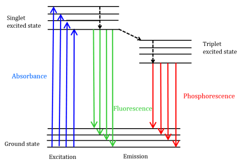
Fluorescent molecules can also undergo there are three methods of nonradiative relaxation where the excitation energy is not converted into photons: (1) internal conversion, (2) external conversion, and (3) intersystem crossing.
(1) Internal conversion occurs when there is a relatively small energy gap between two electronic states and the electrons transition from a higher electronic state to one of lower energy. Here the energy is transferred to the vibrational modes of the electronic state. Since vibrational processes are thermally driven, increasing temperature leads to decreases in fluorescence intensity.
(2) In external conversion, energy is lost through collisional quenching with solute molecules in the fluorophore’s environment.
(3) Intersystem crossing arises when vibrational levels of the singlet and triplet excited states overlap in energy and electrons transition from the lowest singlet excited state to the first excited triplet state. The photons emitted as they return back to the ground state is known as phosphorescence (Figure 1). The triplet state is lower in energy than the singlet state so phosphorescence peaks are found at longer wavelengths than fluorescence. Since these transitions are also forbidden, phosphorescence exhibits a longer lifetime (~10-4 – 102 seconds) compared with fluorescence (~10-9 – 10-6 seconds). The longer lifetimes also lead to thermal deactivation via oxygen quenching, solvent movement, and intermolecular collision so phosphorescence typically cannot be observed at room temperature and samples must therefore be cooled at liquid nitrogen temperature.
Principle of Measurement
In emission spectroscopy the light detected is not from the lamp, but instead is emitted from the sample. When the sample emits light it does not preferentially emit in a particular direction meaning not all emitted light reaches the detector. This means the levels of light are substantially lower than a UV-Vis making limitation of noise a high priority. The intensity of emission also relates directly to the intensity of the lamp hitting the sample meaning that greater S/N can be achieved if more light hits the samples. However, this direct correlation can cause issues when making comparisons between excitation wavelengths. See our instrument theory page for more info on this.
Advantages of Fluorescence Spectroscopy
Fluorescence spectroscopy offers the following advantages:
- High sensitivity
Absorption spectroscopy detects decreases in incident light intensity, whereas fluorescence spectroscopy detects the intensity of emitted light. It is highly sensitive because it detects the difference from zero light intensity.
- High selectivity
Specific fluorescent labeling is possible by binding fluorescent molecules to the target molecules. This is why fluorescence analysis is considered highly selective.
- High environmental dependency
The shape and intensity of the fluorescence spectrum are sensitive to the environment surrounding the fluorescent molecules (solution pH, temperature, solvent type, coexisting salt). This can be used to probe the surrounding environment.
Beer’s Law and Concentration Effects
While absorption occurs on the timescale of less than 10-15 seconds, the relaxation process from the excited to the ground state is much slower. Therefore, fluorescence can provide information on a fluorophores’ interactions with surrounding molecules and solvents, unlike absorption.
Fluorescence intensity is directly proportional to the excitation light intensity
F=2.303 * K * I0 * εbc
where K is a constant based on instrument geometry, I0 is the intensity of the excitation light, ε is the fluorophore’s molar absorptivity, b is the pathlength, and c is the concentration. Since the fluorescence intensity is not ratioed to the incident light intensity like with absorption measurements, the fluorescence sensitivity is much greater because it is not limited by the instruments ability to differentiate between the incident and detected intensities. Consequently, smaller concentrations are required for measurements.
The above equation is only applicable when the sample absorbance is less than 0.05 O.D. If a sample is too concentrated, the emission light can be reabsorbed by the fluorophore, attenuating the fluorescence signal at shorter wavelengths. Excitation light may also not fully penetrate the full width of a highly concentrated sample, which will also lead to decreased fluorescence intensities.
Why Use Fluorescence Spectroscopy?
Advantages
- High sensitivity enables detection of very low analyte concentrations because emitted light is measured against a near-zero background signal.
- Only looking at fluorescent molecules enables targeting of specific fluorophores or fluorescent labels to target compounds of interest in complex samples.
- Environmental responsiveness makes fluorescence spectroscopy useful for monitoring changes in pH, polarity, temperature, molecular binding, and conformational structure.
- Rapid, non-destructive analysis supports applications in life science, pharmaceutical, environmental, and materials characterization.
Limitations
- Photobleaching may reduce fluorescence intensity over time as fluorophores degrade during prolonged light exposure.
- Inner-filter effects can distort fluorescence intensity and spectral shape when highly absorbing or concentrated samples reabsorb excitation or emission light.
- Matrix interferences and scattering artifacts such as Rayleigh and Raman scatter may introduce background signals and spectral distortion.
- Sensitivity to experimental conditions means fluorescence signals can vary with solvent composition, temperature, pH, and sample contaminants.
Who Should Use Fluorescence Spectroscopy?
- Biotechnology and Life Science Research
Fluorescence spectroscopy is commonly used for nucleic acid quantification, protein characterization, enzyme kinetics, and cell-based assays. For example, fluorescein-labeled biomolecules are typically measured at excitation wavelengths near 490 nm with emission near 520 nm, while intrinsic protein fluorescence from tryptophan residues is often monitored using excitation around 280 nm and emission near 350 nm. - Pharmaceutical and Clinical Diagnostics
In pharmaceutical analysis and clinical laboratories, fluorescence methods support drug discovery, biomarker detection, immunoassays, and therapeutic monitoring. Fluorescent probes used in diagnostic assays may operate within excitation ranges of 350–500 nm and emission ranges of 450–650 nm depending on the fluorophore and target analyte. - Environmental Analysis
Environmental laboratories use fluorescence spectroscopy to detect pollutants, dissolved organic matter, hydrocarbons, and trace contaminants in water and soil samples. Polycyclic aromatic hydrocarbons (PAHs), for example, commonly exhibit excitation wavelengths in the UV region around 250–380 nm with emission between 300–500 nm. - Materials Science and Nanotechnology
Fluorescence spectroscopy is used to characterize polymers, semiconductors, nanoparticles, and quantum dots by evaluating electronic and optical properties. Quantum dots often display broad excitation ranges with size-dependent emission wavelengths spanning approximately 450–700 nm. - Food and Agricultural Testing
Fluorescence analysis can identify vitamins, toxins, contaminants, and quality indicators in food products and agricultural samples. Riboflavin, for example, is frequently analyzed using excitation near 450 nm and emission near 530 nm. - Chemical and Industrial Analysis
Industrial laboratories use fluorescence spectroscopy for process monitoring, dye analysis, forensic investigations, and chemical identification. Fluorescent tracers and optical brighteners are commonly analyzed using excitation wavelengths in the UV-to-visible range with emissions selected according to compound-specific fluorescence characteristics.
Instrumentation of Fluorescence Spectroscopy
How it Works
Generally fluorescence is measured from an instrument as follows:
- Excite the sample A light source, typically a xenon lamp or laser, directs excitation energy onto the sample at a selected wavelength. Fluorophores within the sample absorb this energy and transition from the ground state to an excited electronic state.
- Relax to a lower energy state After excitation, the molecules rapidly lose a portion of their energy through non-radiative relaxation processes such as vibrational relaxation and internal conversion. This occurs within picoseconds to nanoseconds.
- Emit Fluorescence The excited molecules return to the ground state by emitting light at a longer wavelength than the excitation source. This emitted light is the fluorescence signal measured by the instrument.
- Isolate the emission Signal A monochromators separate the fluorescence emission from scattered excitation light. This improves signal-to-noise ratio and ensures only the desired emission wavelengths reach the detector. Spectrofluorometers commonly position the detector at a 90° angle to minimize interference from transmitted excitation light.
- Detect the Fluorescence The isolated fluorescence is measured using highly sensitive PMT detector. These detectors convert the emitted photons into electrical signals proportional to fluorescence intensity.
- Collect excitation or emission spectra The instrument software processes the detected signal to generate fluorescence spectra. Emission spectra are produced by scanning emitted wavelengths at a fixed excitation wavelength, while excitation spectra are obtained by scanning excitation wavelengths while monitoring emission intensity at a fixed wavelength.
Monochromators
Fluorometers are composed of an excitation and emission monochromator, allowing users to obtain both excitation and emission spectra.
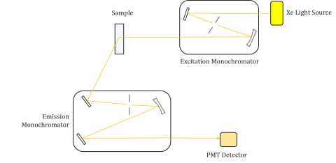
Excitation spectra plot the intensity at a fixed emission wavelength while varying the excitation wavelengths using the excitation monochromator. Since most emission spectra are independent of the excitation wavelength, the excitation spectra are frequently duplicates of the fluorophore’s absorption spectrum.
An Emission spectrum plots the intensity at a fixed excitation wavelength while scanning through varying emission wavelengths using the emission monochromator. These emission scans provide information on the molecular structure of the fluorophore and the local environment surrounding it. Since the fluorescence emission always occurs from the lowest excited state to the ground state, the shape of the emission spectrum is usually independent of the excitation wavelength. More energy is also required to excite a molecule from the ground to the excited state, resulting in emission peaks at longer wavelengths (i.e. smaller energies) than their corresponding excitation wavelengths. This difference in energy between the excitation and emission wavelengths is known as the Stokes shift.
In addition, absorption and emission spectra are frequently mirror images of one another due to the equal distribution between the vibrational energy levels of the excited and ground states (Figure 3). The Franck-Condon principle explains that because the nuclei are relatively large and the electronic transition involved in emission and absorption occur on such fast time scales, there is no time for nuclei to move and the vibrational energy levels and therefore remain roughly the same throughout the electronic transition.

Gratings
The dispersive element used in emission spectrometers is a grating. This provides linear dispersion of wavelengths, but also leads to preference for a specific polarization, either vertical or horizontal.
G-factor
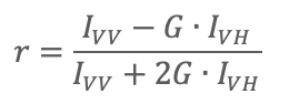
Fluorescence instruments will have inherent bias towards detection of vertically or horizontally polarized light. This is often called G factor where G=2 would indicate that the system detects vertically polarized light twice as well as horizontally. This factor is essential to know for anisotropy experiments which rely on the use of polarized light for excitation and emission. The G factor can be calculated as

Where IHV is the intensity of detected light with horizontal excitation and vertical emission polarization and IHH is the intensity of detected light with horizontal excitation and horizontal emission polarization. This factor can then be applied to get true total fluorescence intensity

And true fluorescence anisotropy
Spectral Correction
Like UV-Visible absorption spectroscopy, fluorescence spectroscopy relies on the detection of light after a lamp irradiates a sample. However, there is a key distinction which makes fluorescence spectroscopy different. For UV-Vis the quantity being determined is often absorbance which is given by the following equation
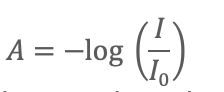
Where I is the intensity of light after the sample and Io is the light intensity before the sample or if the sample is not present. This quantity A is ratiometric, meaning that if the lamp is higher intensity (Io is higher) then the light after the sample (I) is also higher, cancelling any lamp contribution to the signal. This allows for direct comparison between two different UV-Vis systems which in turn give identical Absorbance values.
In a fluorometer the detector is off axis from the excitation source and only takes in light emitted or scattered from the sample. This means fluorescence is directly related to luminous flux the lamp and the efficiency of the detector. Components such as the light source, monochromator optics, and photomultiplier tube therefore directly impact fluorescence signal intensity as a function of wavelength. This means a measurement made by a fluorometer is unique to the individual instrument’s excitation and emission monochromators.
Spectral Bandwidth
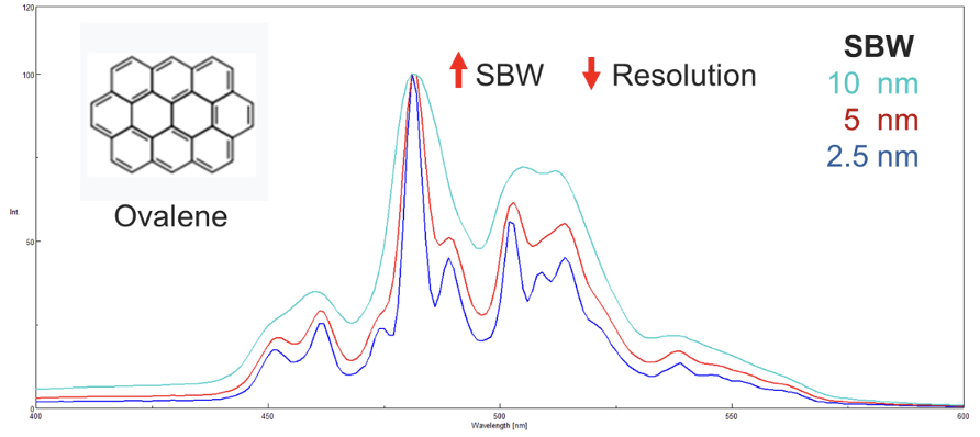
Since the fluorescence intensity is proportional to the input light intensity, the amount of light passed through the monochromator will greatly affect the intensity. The sum of the excitation and emission bandwidths should be about the spectral bandwidth (SBW) of the peak being monitored so that all peaks are well resolved. As long as this rule of thumb is followed, the bandwidths can be opened to increase the amount of light throughput for samples with low fluorescence. The SBW can also be impacted by the Stokes shift of the fluorophore. Narrower Stokes shifts may limit the range of acceptable SBWs that can be used.
Fluorescence Artifacts
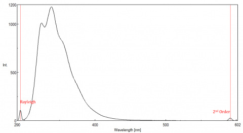
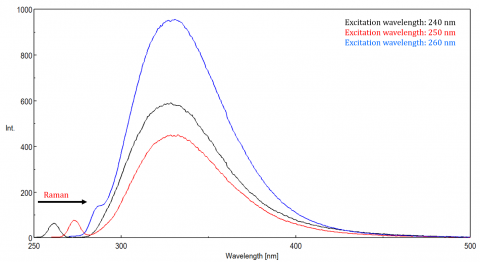
Scattered light can give rise to artifacts, distorting the fluorescence spectrum. The three most common types of scatter seen in fluorescence are Rayleigh, 2nd order, and Raman scatter (Figure 4). Rayleigh scattering is the scattered excitation light and therefore peaks at the excitation wavelength. 2nd order scatter is higher-order scatter observed at twice the excitation wavelength (if exciting at 300 nm, a peak is seen at 600 nm). Raman scattering is inelastic scatter due to solvents and peaks at a fixed energy from the excitation wavelength. To differentiate Raman scattering from a fluorescence peak, the excitation wavelength can be varied in 5 to 10 nm increments and if the peak in question shifts with the excitation wavelength and decreases in intensity, then that peak, is due to Raman scatter. You can also check to see if the peak is in the blank solvent spectrum. If it is, there is a chance it is a Raman peak. If the fluorescence peak is too close or overlapping with either the Raman or Rayleigh scatter, the bandwidths and/or excitation wavelength can be adjusted to shift the scatter off the fluorescence peak. These effects are most prominent for very low fluorophore concentrations and especially highly scattering solutions, like proteins, microsphere, nanoparticles, as well as solids.
Dynamic Range
The Automatic Gain Control function automatically adjusts the gain of a signal from the detector based on the fluorescence intensity. This optimizes the signal to noise throughout the entire scanned range for spectral or time course measurements so that peaks with different intensities are automatically adjusted to improve the S/N and assure result accuracy.
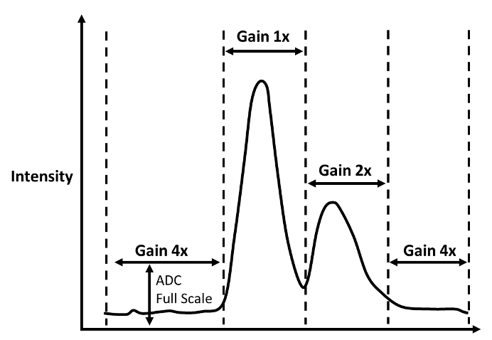
Automatic Sensitivity Control System (SCS)
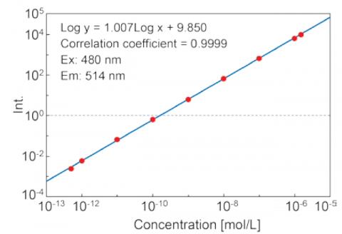
The Automatic Sensitivity Control System (SCS) expands the dynamic range of the detected fluorescence signal by automatically adjusting the detector voltage according to the fluorescence intensity. This allows for fixed wavelength or quantitative analyses measurements of sub-picomolar to micromolar concentrations without manually changing the instrument.